Probabilistic 2-meter surface temperature forecasting over Xinjiang based on Bayesian model averaging

1 Introduction

The Xinjiang Meteorological Service has recently strengthened the construction of a fine grid forecast platform based on multi-model forecasts. However, due to the uncertainty of initial field data and model parameters, meteorological factors such as temperature and precipitation forecast by numerical models differ from the observations. There are also differences in the forecast of meteorological elements such as temperature among model products, making it difficult for a single model product to fulfill the actual forecast needs (Cai and Yu, 2019; Peng and Zhi, 2019).

Forecasts based on multi-model ensembles can improve the performance of model prediction and be used in probabilistic forecasts. Many studies have investigated the Bayesian model averaging (BMA) method based on ensemble forecasts (Tan and Jiang, 2016; Ji et al., 2019; Lee and Shin, 2020). For example, Raftery et al.(2005) applied the BMA method to the ensemble of dynamic meteorological models for the first time to forecast normal variable temperature and sea level pressure and found that the performance of the BMA method was significantly better than that of the traditional ensemble mean method, and the root mean square error (RMSE) of the BMA method was 8% lower than that of the ensemble mean method. Zhiand Wang(2015) used the BMA method to estimate the temperature in East Asia from 2011 to 2035. They pointed out that the temperature generally increased under the representative concentration pathway 4.5 (RCP4.5) scenario, and the increase in the ocean was relatively small. Ji and Zhi(2017) studied the extension period forecast of 2-m temperature in East Asia via the BMA method and concluded that the BMA method significantly improved the ensemble forecast performance.

Additionally, the BMA method is better than the traditional method in simulating observations and can reduce the uncertainty of model simulation. Miao et al. (2014) used the BMA method, simple model averaging, and reliability ensemble averaging (REA) to evaluate the ability of the coupled model intercomparison project phase 5 (CMIP5) model on interannual and interdecadal changes in the surface temperature in Eurasia. The results demonstrated that the BMA and REA methods significantly improved the ability of model simulation, and the BMA method had the lowest uncertainty. Brunner et al. (2020) and Zhao et al. (2020) have pointed out that compared with traditional methods, the BMA method can better reduce the deviation between the model and observation and better capture uncertainty and local climate features. In the statistical downscaling of large-scale variables, Zhang and Yan(2015) pointed out that the downscaling method combining the optimum correlation method and the BMA method has a better performance than multiple linear regression. Fang and Li(2016) estimated the uncertainty, weight, and variance of the paleoclimate modeling intercomparison project phase 3 (PMIP3) and CMIP5 model simulations by using the BMA method. They found that the BMA method considers the simulation capability of different models and generates more reliable past time variations over long periods based on multi-model ensembles and training sets. Javanshiriet al(2021) noted that the BMA method was more accurate, skilled, and reliable than the ensemble model output statistics-censored shifted gamma method and had better resolution but poor discrimination in predicting the probability of high precipitation events.

The terrain of Xinjiang is relatively complex. The regional numerical model assimilates local observation data and satellite data, which can better simulate and forecast extreme weather, and has advantages in forecasting some small-scale regions. However, due to the limitation of computing resources and storage space, the current regional numerical model can only provide deterministic forecasting results. In addition, the forecasting results of global numerical models such as the ECWMF model are relatively stable but cannot simulate and forecast extreme weather well. Therefore, in this study, global numerical models are combined with regional models to investigate the probabilistic forecasts of 2-m temperature in Xinjiang, China, using the BMA method. Section 2 introduces observations and four model products. Section 3 introduces the BMA method. Section 4 selects the best training period of the BMA model, analyzes the temporal and spatial characteristics of BMA deterministic and probabilistic forecasts, and evaluates the BMA forecast performance. Section 5 and Section 6 provide the discussion and main conclusions, respectively.

2 Data and methods

2.1 Data

The 24 h 2-m temperature forecasts (initialized at 0000 UTC) from May 30 to 31 August 2020, used in this study were obtained from the Xinjiang regional weather forecast system Desert Oasis Gobi Regional Analysis Forecast System (DOGRAFS) and Rapid-Refresh Multiscale Analysis and Prediction System (RMAPS) developed by the Urumqi Institute of Desert Meteorology of China Meteorological Administration, the European Center for Medium-Range Weather Forecasts (ECMWF), and the China Meteorological Administration–Global Forecast System (CMA-GFS) (Zhang and Chen, 2012).

DOGRAFS, which achieved business access in 2015, is based on the weather research and forecast (WRF) model and WRF data assimilation (WRFDA) in version 3.5.1, with triple nested domains and 40 vertical computational layers. The regional resolution of Xinjiang is 9 km, and the regional resolution of Urumqi to Xiaocaohu is 3 km. The atmospheric and surface fields of the National Centers for Environmental Prediction (NCEP) GFS model forecasts were introduced as the initial conditions. The RMAPS is based on the WRF model and WRFDA in version 4.1.2, with two nested domains and 50 vertical computational layers. For the Central Asia region and Xinjiang, China, the regional resolutions are 9 km and 3 km, respectively. The RMAPS takes the atmospheric and surface fields of the NCEP GFS model forecasts as the initial conditions and realizes trial operation at the end of May 2018 (Ju and Liu, 2020; Tang and Li, 2021).

All forecasts are interpolated to 103 observation stations over Xinjiang, China, to evaluate the performance of the BMA method and different model products and their ensemble mean. Figure 1 shows the orographic effects of the study area and the location of observation stations. It can be seen that the distribution of observation stations in the study area is not uniform, and the terrain is complex. In addition, southern Xinjiang is subjected to drought, with large diurnal temperature differences and complex climatic characteristics (Yao et al., 2022). Furthermore, the topography of the initial field of the numerical model is different from the actual topography. All of these factors may have an impact on BMA forecast results (Liu and Ju, 2020; Xin and Li, 2021).

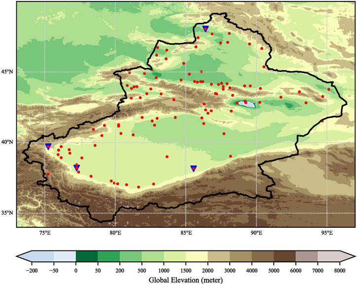
FIGURE 1. Orographic effects of the study area and the location of observation stations. The blue inverted triangles represent the example stations of X51053, X51705, X51815, and X51855.

2.2 Methods

BMA is a statistical post-processing method for multi-model ensemble forecasts. Its basic principle is to take a weighted average of multi-model forecasts instead of selecting the best members (Raftery et al., 2005). Assuming that $y$ is the predictor, $y^T$ is the observation data during the training period, $f_k\left(k=1,\dots ,K\right)$ is the forecast result of $K$ model products, and the probability density function (PDF) of the BMA model is given by

where $p\left(y|f_k\right)$ is the conditional probability of predictor $y$ based on model $f_k$, $p\left(f_k|y^T\right)$ is the posterior probability of $y$ forecasted by model $f_k$ for a given $y^T$, and ${\displaystyle \sum }_k^{K}p\left(f_k\text{|}{y}^T\right)=1$. In essence, the BMA method uses $p\left(f_k\text{|}{y}^T\right)$ as the weight of model $k$. Therefore, the PDF of the BMA model can be expressed as

where ${\omega }_k$ represents the relative contribution of model $k$ to the forecast (i.e., the weight of model $k$), and ${\displaystyle \sum }_k^K{\omega }_k={\displaystyle \sum }_k^{K}p\left(f_k\text{|}{y}^T\right)=1$.

For surface temperature forecasting, the normal linear hypothesis with expectation $a_k+b_k{f}_k$ and variance ${\sigma }_k$ can be adopted:

where $a_k$ and $b_k$ can be obtained from the linear relationship between observation $y^T$ and forecast $f_k$. Under this assumption, the conditional expectation of predictor $y$ is the mean value of the BMA forecast:

Eq. 4 can be understood as a deterministic forecast, which can be compared with the mean value of the multi-model ensemble mean or a single-model forecast.

Under the assumption of normal linearity, parameters of the BMA model were solved by using the observation and model data in the training period. For predictor, the estimates of $a_k$ and $b_k$ can be regarded as a simple deviation correction process. The weights and variance ${\sigma }_k$ can be estimated using the log-likelihood function. Assuming that the forecast error is independent of space (different stations) and time (different forecast times), the log-likelihood function of the BMA model is provided by

where $N$ represents the length of the training period, and $s$ and $t$ represent station $s$ and time $t$, respectively. When Eq. 5 estimates the conditional distribution of predictor $y$ based on model $f_k$ (i.e., when a single predictor y is estimated), there is no analytical maximum. Therefore, the expectation-maximization algorithm is used to solve the parameters.

In addition, this study uses the continuously ranked probability score (CRPS), forecast accuracy, relative error analysis, Brier score (BS), RMSE, and Taylor diagram to evaluate the correction and performance of the BMA method on multi-model ensembles.

The CRPS of the multi-model ensemble mean can be written as

where $X$ and $X$ are independent copies of a random variable with the distribution function $F$ and finite first moment (Gneiting and Raftery, 2007).

The forecast accuracy can be expressed as

where $f_{st}$ and the $y^{st}$represent the forecast and observation of the station $s$ during the time $t$, respectively (Cui and Peng, 2002).

Assuming that $P_{mi}$ and $P_{oi}$ are the probabilities of numerical models (or BMA forecasts) and observations within the ith interval and $k$ is the number of separated intervals (Fu et al., 2013), then the BS is given by

3 Results

3.1 Selection of the best training period

The BMA method needs to divide data into training and forecast periods, and the length of the training period affects the BMA forecast results (Zhi and Peng, 2018). Therefore, before forecasting the 2-m temperature in the Xinjiang region, determining the best training period for the BMA model is necessary. Because the data duration was 92 days, the first 70 days were selected to participate in the sliding training. The best training period was selected from 41 to 70 days. Figure 2 shows the CRPS scores and RMSEs for different training periods. The CRPS score and RMSE showed the same trends. Before 47 days, the CRPS score and RMSE decreased, but after 47 days, they continued to increase. When the training period was 47 days, the CRPS score and RMSE were the minimum. Therefore, 47 (from June 1 to July 17) days were selected as the training period of the BMA model to conduct deterministic and probabilistic forecasts of 2-m temperature, and the remaining 45 (from July 18 to August 31) days were used to evaluate the BMA forecast and multi-model ensembles (i.e., forecast period).

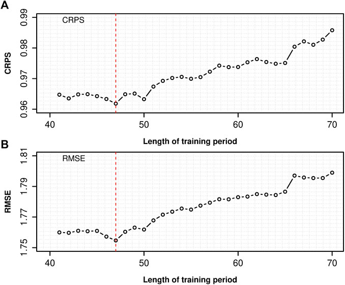
FIGURE 2. Verification metrics of (A) CRPS score and (B) RMSE with different training period lengths for the BMA forecast.

Additionally, to demonstrate the contribution of each model to the 2-m temperature forecast under different training periods, Figure 3 shows a boxplot of the weights of the four models in the sliding training periods. Except for ECMWF, the weights of the other three models change little at different training periods, indicating that each model has a relatively stable contribution to 2-m temperature prediction at different training periods. The weight of the ECMWF remained 0.6–0.7, the RMAPS weight was less than 0.1, and the DOGRAFS and CMA-GFS weights were 0.1–0.15. This result indicates that among the 2-m temperature forecasts of 103 stations in Xinjiang, ECMWF forecast information is dominant, followed by DOGRAFS, CMA-GFS, and RMAPS.

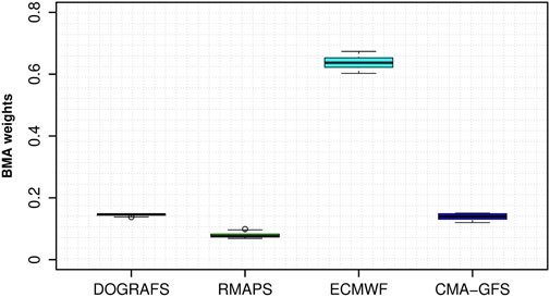
FIGURE 3. Boxplot of weights of four models under different training periods for the BMA forecast.

3.2 Probability forecast of Bayesian model averaging

After selecting the best training period, the deterministic prediction results of the BMA forecast and multi-model ensembles were analyzed. The forecasting performance of the same numerical model at different stations is quite different, and different numerical models have different forecasting performances at the same station. Furthermore, the BMA forecasting error of most stations is within 2°C, but the BMA forecasting error of some stations is more than 2°C. Therefore, in order to compare the results of observation, BMA probabilistic forecast, BMA deterministic forecast, and different numerical model forecasts, four stations where there are great differences among different forecast results are selected as representative stations. Figure 4 shows the BMA probability forecast curve, BMA deterministic forecast, and different model deterministic forecasts and their ensemble mean values of 2-m temperature with a lead time of 24 h at four representative stations. Representative station X51053 is an example (Figure 4A): the observed 2-m temperature is 23.7°C (solid gray line in Figure 4A); the maximum and minimum errors of the four models are 4.9°C and 0.63°C, respectively (solid green and blue lines in Figure 4A); and the prediction error of the multi-model ensemble mean also reached 3.1°C (solid black line in Figure 4A). After the multi-model forecasts are processed by the BMA method, the error between the BMA deterministic forecast and observation is 1°C.

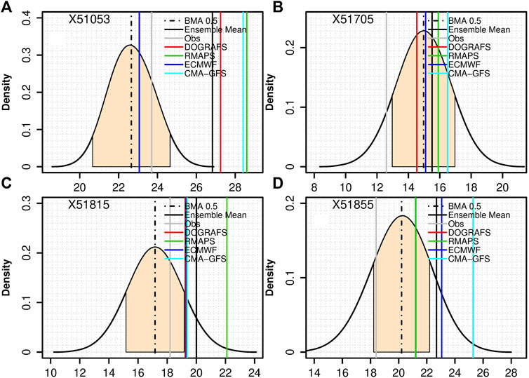
FIGURE 4. Deterministic forecasts and BMA probability forecasts of 2-m temperature at stations (A) X51053, (B) X51705, (C) X51815, and (D) X51855 with a lead time of 24 h. The black curve and black dotted line represent the BMA probability forecast curve and deterministic forecast curve, respectively. Gray and black solid lines represent the observed and multi-model ensemble mean deterministic forecasts; the remaining solid lines represent the deterministic forecasts of the four models. The shadow represents the probability centered on the BMA deterministic forecast with an interval length of 2°C.

For representative stations X51705, X51815, and X51855, although the minimum error of each model and multi-model ensemble means for the 2-m temperature forecast was 1°C, there were significant differences among the models, and the maximum forecast error reaches 6.9°C. Moreover, the same model had different forecasting performances at different stations. The maximum error of the deterministic BMA forecast weighted by the four models is approximately 2°C, indicating that the BMA method can effectively reduce the error of the observation and model forecasts. Additionally, except for the X51705 station, the observation of the other three representative stations basically falls within the uncertainty range (i.e., the solid gray line is in the shadow). As shown in Figure 4, with the larger interval (i.e., the PDF is flatter), there is a larger possibility that the observation (gray line in Figure 4) is to fall in the interval. In other words, the forecast uncertainty is lower.

To further analyze the regional characteristics of BMA probability forecast uncertainty (i.e., the probability that the forecast error is within 2°C), Figure 5 shows the spatial distribution of 2-m temperature uncertainty with a lead time of 24 h in Xinjiang (i.e., the probability distribution centered on the BMA deterministic forecast of each station and with an interval length of 2°C). The probability of most stations in Xinjiang exceeded 0.6. Among them, the probability of most stations in southern Xinjiang is 0.6 ∼ 0.8 and of some stations is less than 0.6. The probability of most stations in northern Xinjiang is more than 0.7, and the probability of stations in western northern Xinjiang is 0.9–1. This result shows that forecast uncertainty in southern Xinjiang is greater than that in northern Xinjiang. In other words, from low latitude to high dimension, the 2-m temperature uncertainty of the BMA forecast in Xinjiang decreases.

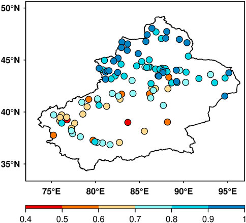
FIGURE 5. Spatial distribution of 2-m temperature uncertainty of the BMA forecast at each station. (i.e., probability distribution with the BMA deterministic forecast as the center and interval length of 2°C).

3.3 Evaluation of the Bayesian model averaging forecast

According to the aforementioned analysis, different models have different forecast performances on four stations, and the BMA method effectively reduces the forecast error between the observation and models. To compare the performance of the multi-model ensemble mean and BMA forecast for each station, Figure 6 shows the CRPS score of the multi-model ensemble mean and BMA forecast. There are significant differences in the CRPS scores of the multi-model ensemble mean at each station. Among them, the CRPS scores of some stations in central Xinjiang exceeded 4, and some stations exceeded 7. The CRPS scores of other stations were approximately 1–4 and those of some stations were lower than 1 (Figure 6A). In the spatial distribution, the simple ensemble mean method has poor prediction performance, and the CRPS scores differ. The CRPS score of the BMA forecast of some stations was less than 2, and the CRPS score of most stations was less than 1 (Figure 6B). This shows that the forecast performance of the BMA method is better than that of the multi-model ensemble mean. Additionally, the overall prediction performance of the BMA method for spatial distribution is consistent.

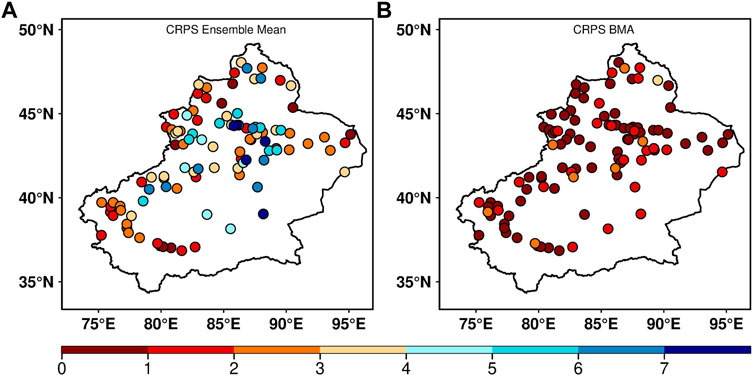
FIGURE 6. Spatial distribution of the CRPS score for (A) multi-model ensembles and (B) BMA forecast of 2-m temperature with a lead time of 24 h.

Figure 7 shows the spatial distribution of RMSE between the observation and BMA deterministic forecasts, four models, and their multi-model ensemble mean in the forecast period. During the forecast period, the RMSE between the observation and DOGRAFS, RMAPS, and CMA-GFS forecasts was above 2°C for most stations in Xinjiang (Figures 7C,D,andF). Among them, the RMSE of the RMAPS forecast at some stations exceeded 3°C, and the RMSE of the CMA-GFS forecast exceeded 5°C. The RMSE between the observation and ECMWF forecast is between 1°C and 4°C at most stations (Figure 7E). Among them, the RMSE of stations in the northwest of northern Xinjiang is between 1 and 3°C. Additionally, the RMSE between the observation and multi-model ensemble mean is between 2°C and 5°C at most stations (Figure 7B). The RMSE between the observation and BMA forecast is reduced to less than 2°C at most stations, and at some stations, it is between 2°C and 3°C. In other words, there is a large forecast error between the observation and the CMA-GFS forecast at most stations in the forecast period, and the forecast error of the other three models remains between 2°C and 5°C. In addition, the multi-model ensemble mean does not reduce the forecast error between the observation and the model. The error between the observation and the BMA forecast in the forecast period was lower than that of each model, and there was no obvious regional difference.

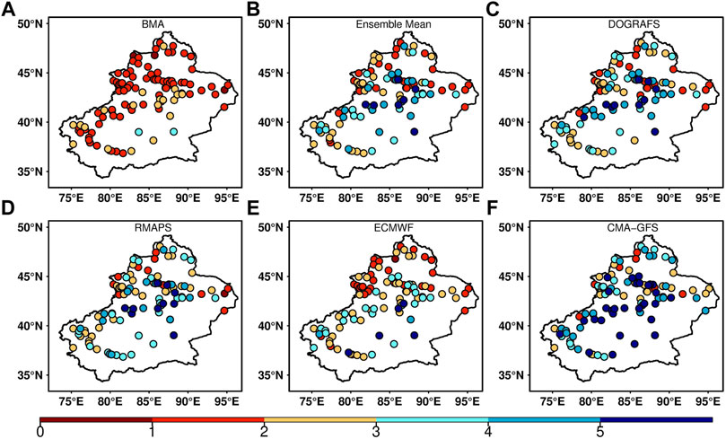
FIGURE 7. Spatial distribution of RMSE between (A) BMA, (B) multi-model ensemble mean, (C) DOGRAFS, (D) RMAPS, (E) ECMWF, (F) CMA-GFS and observed 2-m temperature during the forecast period.

Furthermore, Figure 8 shows the box plot of the Brier score, relative error and forecast accuracy of BMA forecast, and different model forecasts of 2-m temperature at observation stations during the forecasting period. As shown in Figure 8, the distribution of Brier score, relative error, and forecast accuracy of single model forecasts are scattered, which means that the accuracy of single model forecasts at different stations is significantly different in the forecasting period. During the forecasting period, the distribution of the Brier score, relative error, and forecast accuracy of BMA forecasts is concentrated. The Brier score and relative error of most stations are also close to 0, and the median forecast accuracy is close to 0.8. Compared with a single model forecast, the accuracy of BMA forecasts is basically consistent in spatial distribution better than single model forecasts.

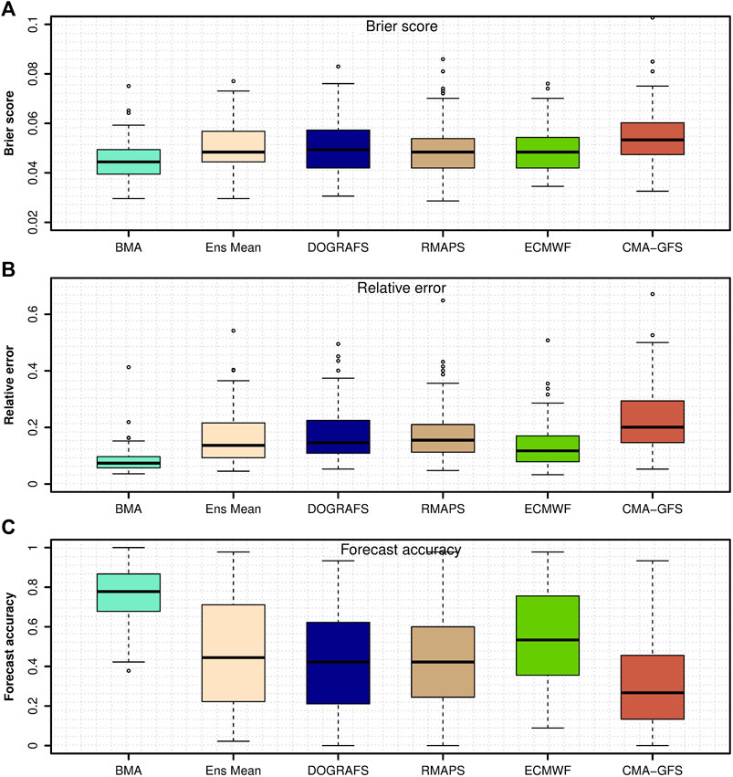
FIGURE 8. Box plot of the (A) Brier score, (B) relative error, and (C) forecast accuracy analysis of the BMA forecast and different model forecasts of 2-m temperature at observation stations during the forecasting period.

In addition, to make a more intuitive comparison between the BMA forecast and different models’ (and multi-model ensemble mean) forecasts of 2-m temperature in the Xinjiang, Figure 9 shows the Taylor diagram of the forecasts and observation (the mean of the forecast period at each station). The distance from different forecasts to the observation (the hollow point on the abscissa) represents the RMSE of the observation and forecast. The distance from different forecast results to the origin of the coordinate represents the ratio of the standard deviation of the forecast and observation. The angle between different forecasts and the horizontal axis represents the correlation coefficient between forecast and observation. The abscissa represents the correlation coefficient of forecast and observation. The correlation coefficient between the deterministic forecast of the four models, and the observation is approximately 0.9, RMSE is above 0.5, and the ratio of standard deviation exceeds 1. Compared with the forecast of each model, the multi-model ensemble mean only improves in correlation. However, the standard deviation and correlation coefficient between the BMA forecast and observation were over 0.98, and the RMSE decreased significantly.

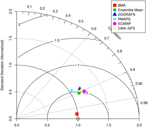
FIGURE 9. Taylor diagram of BMA and multi-model forecast of 2-m temperature during the forecast period.

These results indicate that the 2-m temperature forecasts of the four models and their ensemble mean differ from the observations in dispersion degree and spatial distribution. The BMA method significantly reduces the difference, and its forecast is closer to the observation.

4 Discussion

Notably, the regional numerical models adopted in this study are the forecast products commonly used by the Xinjiang Meteorological Bureau for daily weather forecasting. In this study, we evaluated the performance and error of four models for 2-m temperature forecasts in the Xinjiang region while conducting probability forecasts based on the BMA method. In general, the ECMWF was better than the other three regional numerical models. Additionally, the deterministic forecast of the 2-m temperature in Xinjiang by different models is inconsistent in different regions. The BMA method makes up for the spatial uniformity of the model forecast, effectively reduces the RMSE of the model forecast and observation, and provides probabilistic prediction results.

In addition, BMA forecast reliability (forecast uncertainty) can be judged using the BMA deterministic forecast and probability forecast results. Zhi and Peng(2018) and Peng and Zhi(2019) have studied the 2-m temperature probability forecast in different seasons in East Asia and pointed out that the forecast uncertainty of land is greater than that of marine areas and that of high-latitude areas is greater than that of low-latitude areas. In the forecast of 2-m temperature in Xinjiang, the uncertainty of the BMA forecast in southern Xinjiang is greater than that in northern Xinjiang, which may be caused by drought and the desert in southern Xinjiang.

5 Conclusion

In this study, first, based on the deterministic forecasts of the DOGRAFS, RMAPS, ECMWF, and CMA-GFS models, an analysis of the applicability of the BMA method for 2-m temperature forecasts in Xinjiang, China, was conducted. Second, the deterministic and probabilistic forecast characteristics of the BMA method were discussed, and the BMA forecast and different models (and their ensemble mean) were evaluated and compared. The results showed the following:

(1) During the sliding training period, the CRPS score and RMSE exhibited the same trend. The CRPS score and RMSE decreased before day 47 but increased after day 47. Therefore, 47 days was the training period selected for the BMA model. In addition, the contribution of each model to the 2-m temperature forecast was relatively stable under different training periods. Among them, the weight of ECMWF basically remains 0.6–0.7, and the weight of the other models is below 0.15.

(2) Although the minimum error of each model and multi-model ensemble means for the 2-m temperature forecast of the four representative stations is only 0.63°C, there is a difference in the forecast of each model, and the maximum forecast error reaches 6.9°C. Moreover, the same model had different forecasting performances at different stations. However, the maximum error of the BMA forecast is only approximately 2°C, which effectively reduces the error of observation and model forecast. Regarding the uncertainty of the forecast, the probability of most stations in southern Xinjiang is 0.6∼0.8, and the probability of most stations in northern Xinjiang is above 0.7, indicating that the uncertainty of the BMA forecast in southern Xinjiang is greater than that in northern Xinjiang.

(3) Spatial distribution of the CRPS score of the multi-model ensemble mean was significantly different, with the CRPS score ranging from 1 to 7. The CRPS score of the BMA method at each station was below 2, indicating that the overall forecast performance of the BMA method is consistent in space. During the forecast period, the RMSE of the observations and the four model forecasts at most stations were above 2°C, and the largest RMSE exceeded 5°C. However, the RMSE of the observations and BMA forecasts at most stations are within 2°C. In the forecast period, the RMSE of the observation and BMA forecasts were lower than those of the other models, and there was no obvious regional difference. Additionally, the standard deviation and correlation coefficient between the observation and BMA forecasts are more than 0.98, and the RMSE decreases significantly.

Machine learning algorithms such as the support vector machine, light gradient boosting machine, and long short-term memory have been widely used in forecasting meteorological elements (Wang et al., 2018; Fan et al., 2019; Hamid et al., 2020; Qadeer et al., 2020). Compared with machine learning algorithms, statistical post-processing methods such as BMA are relatively easy to model but not sufficiently flexible (Javanshiri et al., 2021). Further research could compare and combine BMA and other statistical methods with machine learning algorithms to evaluate the post-processing methods suitable for Xinjiang. These conclusions provide theoretical support for the post-processing of regional numerical models in Xinjiang.

Data availability statement

The datasets used in this study can be provided by MA (ali@idm.cn) upon request.

Author contributions

All authors contributed to the study's conception and design. Material preparation, data collection, and data curation were performed by, JG, CW, and MS. The methodology and software were performed by WH, LZ and JL. The investigation, visualization, writing—original draft preparation, and analysis were performed by AA, YW, and MA. All authors commented on previous versions of the manuscript. All authors read and approved the final manuscript.

Funding

This work was supported by the China Desert Meteorological Research Fund (Grant No. Sqj2021001), the National Key Research and Development Program (Grant No. 2018YFC1507105), and the National Natural Science Foundation of China (Grant No. 41875023).

Conflict of interest

The authors declare that the research was conducted in the absence of any commercial or financial relationships that could be construed as a potential conflict of interest.

Publisher’s note

All claims expressed in this article are solely those of the authors and do not necessarily represent those of their affiliated organizations, or those of the publisher, the editors, and the reviewers. Any product that may be evaluated in this article, or claim that may be made by its manufacturer, is not guaranteed or endorsed by the publisher.

References

Brunner, L., McSweeney, C., Ballinger, A. P., Befort, D. J., Benassi, M., Booth, B., et al. (2020). Comparing methods to constrain future European climate projections using a consistent framework. J. Clim. 33 (20), 8671–8692. doi:10.1175/jcli-d-19-0953.1
Cai, N., and Yu, J. (2019). Temperature forecasting method based on numerical model bias analysis. Trans. Atmos. Sci. 42 (6), 864–873. (in Chinese). doi:10.13878/j.cnki.dqkxxb.20190305001
Cui, X., Peng, C., Li, J., Liu, X., Xu, S., Wang, Z., et al. (2002). Researches into numerical forecast of hourly temperature in hubei province. Meteorology J. Of Hubei 21 (3), 6–9. (in Chinese). doi:10.3969/j.issn.1004-9045.2002.03.002
Fan, J., Ma, X., Wu, L., Zhang, F., Yu, X., and Zeng, W. (2019). Light Gradient Boosting Machine: An efficient soft computing model for estimating daily reference evapotranspiration with local and external meteorological data. Agric. Water Manag. 225 (C), 105758. doi:10.1016/j.agwat.2019.105758
Fang, M., and Li, X. (2016). Application of bayesian model averaging in the reconstruction of past climate change using PMIP3/CMIP5 multimodel ensemble simulations. J. Clim. 29 (1), 175–189. doi:10.1175/jcli-d-14-00752.1
Fu, G. B., Liu, Z. F., Charles, S. P., Xu, Z., and Yao, Z. (2013). A score-based method for assessing the performance of GCMs: A case study of southeastern Australia. J. Geophys. Res. Atmos. 118 (10), 4154–4167. doi:10.1002/jgrd.50269
Gneiting, T., and Raftery, A. E. (2007). Strictly proper scoring rules, prediction, and estimation. J. Am. Stat. Assoc. 102 (477), 359–378. doi:10.1198/016214506000001437
Hamid, G., Aliakbar, M., and Collins, A. L. (2020). Spatial mapping of the provenance of storm dust: Application of data mining and ensemble modelling. Atmos. Res. 233, 104716. doi:10.1016/j.atmosres.2019.104716
Javanshiri, Z., Fathi, M., and Mohammadi, S. A. (2021). Comparison of the BMA and EMOS statistical methods for probabilistic quantitative precipitation forecasting. Meteorol. Appl. 28 (1), e1974. doi:10.1002/met.1974
Ji, L., Zhi, X., and Zhu, S. (2017). Extended-range probabilistic forecasts of surface air temperature over East Asia during boreal winter. Trans. Atmos. Sci. 40 (3), 346–355. (in Chinese). doi:10.13878/j.cnki.dqkxxb.20161106001
Ji, L., Zhi, X., Zhu, S., and Fraedrich, K. (2019). Probabilistic precipitation forecasting over East Asia using bayesian model averaging. Weather Forecast. 34 (2), 377–392. doi:10.1175/waf-d-18-0093.1
Ju, C., Liu, J., Du, J., Li, H., and Li, M. (2020). Forecast effect comparison test and evaluation of RMAPS-CA in Xinjiang. Desert Oasis Meteorology 14 (3), 68–77. (in Chinese). doi:10.12057/j.issn.1002-0799.2020.03.009
Lee, Y., Shin, Y., Boo, K., and Park, J. (2020). Future projections and uncertainty assessment of precipitation extremes in the Korean peninsula from the CMIP5 ensemble. Atmos. Sci. Lett. 21 (2), 1–7. doi:10.1002/asl.954
Liu, J., Ju, C., Ali, M., Fan, S., and An, D. (2020). The application of C-band Doppler radar ground echo recognition method in Xinjiang. Desert Oasis Meteorology 14 (5), 76–83. (in Chinese). doi:10.12057/j.issn.1002-0799.2020.05.010
Miao, C., Duan, Q., Sun, Q., Huang, Y., Kong, D., Yang, T., et al. (2014). Assessment of CMIP5 climate models and projected temperature changes over Northern Eurasia. Environ. Res. Lett. 9 (5), 055007. doi:10.1088/1748-9326/9/5/055007
Peng, T., Zhi, X., Dong, Y., Wang, Y., and Ji, Y. (2019). Forecast improving of 2-meter surface air temperature in East Asia based on Bayesian model averaging. China Sci. 14 (5), 575–581. (in Chinese). doi:10.3969/j.issn.2095-2783.2019.05.017
Qadeer, K., Rehman, W. U., Sheri, A. M., Park, I., Kim, H. K., and Jeon, M. (2020). A long short-term memory (LSTM) network for hourly estimation of PM2.5 concentration in two cities of South Korea. Appl. Sci. (Basel). 10 (11), 3984. doi:10.3390/app10113984
Raftery, A. E., Gneiting, T., Balabdaoui, F., and Polakowski, M. (2005). Using bayesian model averaging to calibrate forecast ensembles. Mon. Weather Rev. 133 (5), 1155–1174. doi:10.1175/mwr2906.1
Tan, J., Jiang, Z., and Ma, T. (2016). Projections of future surface air temperature change and uncertainty over China based on the Bayesian Model Averaging. Acta Meteorol. Sin. 74 (4), 583–597. doi:10.11676/qxxb2016.044
Tang, Y., Li, R., Ma, Y., Zhang, M., Zhang, J., and Liu, J. (2021). Study on the interpretation and application method of hourly temperature and precipitation forecast based on DOGRAFS. Desert Oasis Meteorology 15 (4), 100–106. (in Chinese). doi:10.12057/j.issn.1002-0799.2021.04.013
Wang, B., Zheng, L., Liu, D. L., Ji, F., Clark, A., and Yu, Q. (2018). Using multi-model ensembles of CMIP5 global climate models to reproduce observed monthly rainfall and temperature with machine learning methods in Australia. Int. J. Climatol. 38 (13), 4891–4902. doi:10.1002/joc.5705
Xin, Y., Li, M., DU, J., Liu, J., Yang, Z., Yang, B., et al. (2021). The development of Xinjiang Meteorology in exploiting data assimilation operational system. Desert Oasis Meteorology 15 (1), 133–143. (in Chinese). doi:10.12057/j.issn.1002-0799.2021.01.018
Yao, J., Chen, Y., Guan, X., Zhao, Y., Chen, J., and Mao, W. (2022). Recent climate and hydrological changes in a mountain – basin system in Xinjiang, China. Earth. Sci. Rev. 226, 103957. doi:10.1016/j.earscirev.2022.103957
Zhang, H., Chen, J., and Long, K. (2012). The study of the impact of dynamical core and physical parameterization scheme on GRAPES-meso forecast error. J. Chengdu Univ. Of Inf. Technol. 27 (2), 202–210. (in Chinese). doi:10.3969/j.issn.1671-1742.2012.02.014
Zhang, X., and Yan, X. (2015). A new statistical precipitation downscaling method with bayesian model averaging: a case study in China. Clim. Dyn. 45 (9-10), 2541–2555. doi:10.1007/s00382-015-2491-7
Zhao, C., Gong, J., Wang, H., Wei, S., Song, Q., and Zhou, Y. (2020). Changes of temperature and precipitation extremes in a typical arid and semiarid zone: Observations and multi-model ensemble projections. Int. J. Climatol. 40 (12), 5128–5153. doi:10.1002/joc.6510
Zhi, X., Peng, T., and Wang, Y. (2018). Extended range probabilistic forecast of surface air temperature using Bayesian model averaging. Trans. Atmos. Sci. 41 (5), 627–636. (in Chinese). doi:10.13878/j.cnki.dqkxxb.20160314001
Keywords: regional numerical model, Xinjiang, 2-m temperature, BMA model, probability forecast
Citation: Aihaiti A, Wang Y, Ali M, Huo W, Zhu L, Liu J, Gao J, Wen C and Song M (2022) Probabilistic 2-meter surface temperature forecasting over Xinjiang based on Bayesian model averaging. Front. Earth Sci. 10:960156. doi: 10.3389/feart.2022.960156
Received: 02 June 2022; Accepted: 04 July 2022;
Published: 15 August 2022.
Edited by:
Jingyu Wang, Nanyang Technological University, SingaporeReviewed by:
Luying Ji, Chinese Academy of Meteorological Sciences, ChinaJunqiang Yao, China Meteorological Administration, China
Copyright © 2022 Aihaiti, Wang, Ali, Huo, Zhu, Liu, Gao, Wen and Song. This is an open-access article distributed under the terms of the Creative Commons Attribution License (CC BY). The use, distribution or reproduction in other forums is permitted, provided the original author(s) and the copyright owner(s) are credited and that the original publication in this journal is cited, in accordance with accepted academic practice. No use, distribution or reproduction is permitted which does not comply with these terms.
*Correspondence: Mamtimin Ali, ali@idm.cn